Diffusion models for removing structured noise

This post is about diffusion models, and how they can be used to remove structured noise from images. Before we dive into diffusion models, we will first very briefly cover the basics of deep generative modeling. Specifically, I would like to start with the manifold hypothesis, and how it can help us understand how generative models are able to learn data distributions. After that, we can delve into diffusion models, and how the score of a distribution comes into play. Lastly, we take a look at how we can apply these models to the very relevant problem of removing structured noise.

Manifold hypothesis

The manifold hypothesis states that many high-dimensional processes lie on low-dimensional manifolds inside this high-dimensional space, the manifold. This means that data that is being described with many variables actually can be effectively represented in a lower dimensional space, embedded within this high dimensional space. This is a very important concept, because it means that we can efficiently learn how the data is distributed by fitting a non-linear lower dimensional manifold to our data points. This is exactly what generative models do. They learn a distribution by modeling lower dimensional representations of data and subsequently formulate a way to generate new data by sampling from that distribution.

Let’s see this in action. Consider an image, which can be represented as an $N$ dimensional random variable $\mathbf{x}$, where each variable represents a pixel $\mathbf{x} = [x_0, x_1, \ldots, x_N]$. See the image below, where the 3D box represents the space of the random variable. In this case, for visibility purposes, it only has $N=3$ dimensions, but in reality, an image with $N$ pixels would have $N$ dimensions.

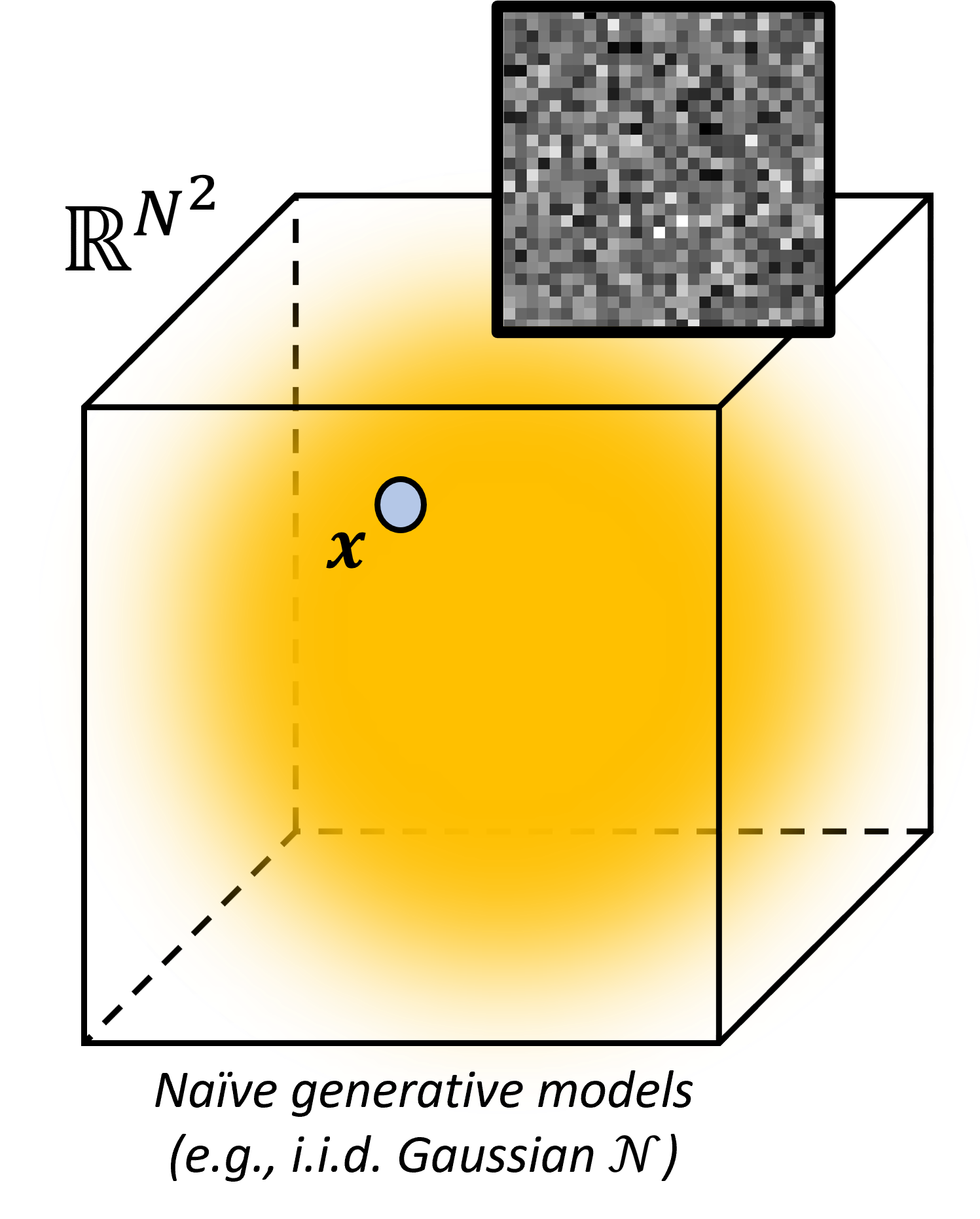
If you would model this random variable as a Gaussian distribution $p(\mathbf{x})\sim\mathcal{N}$, and just sample from that distribution, you would very likely just get random noise. Considering that you are interested in learning a distribution of images of digits, this Gaussian prior would not be a good model for your dataset. The chance of getting an image of a digit, when sampling from a Gaussian distribution, is very low, albeit non-zero. Obviously, we are looking for a more complicated and multimodal model, that can capture the complex distribution of digits. Generative models seek to shape a manifold $\mathcal{M}$, such that it fits to the training data, and puts a higher probability to samples that are similar to your dataset.

A simplified example of such a learned manifold is depicted below.

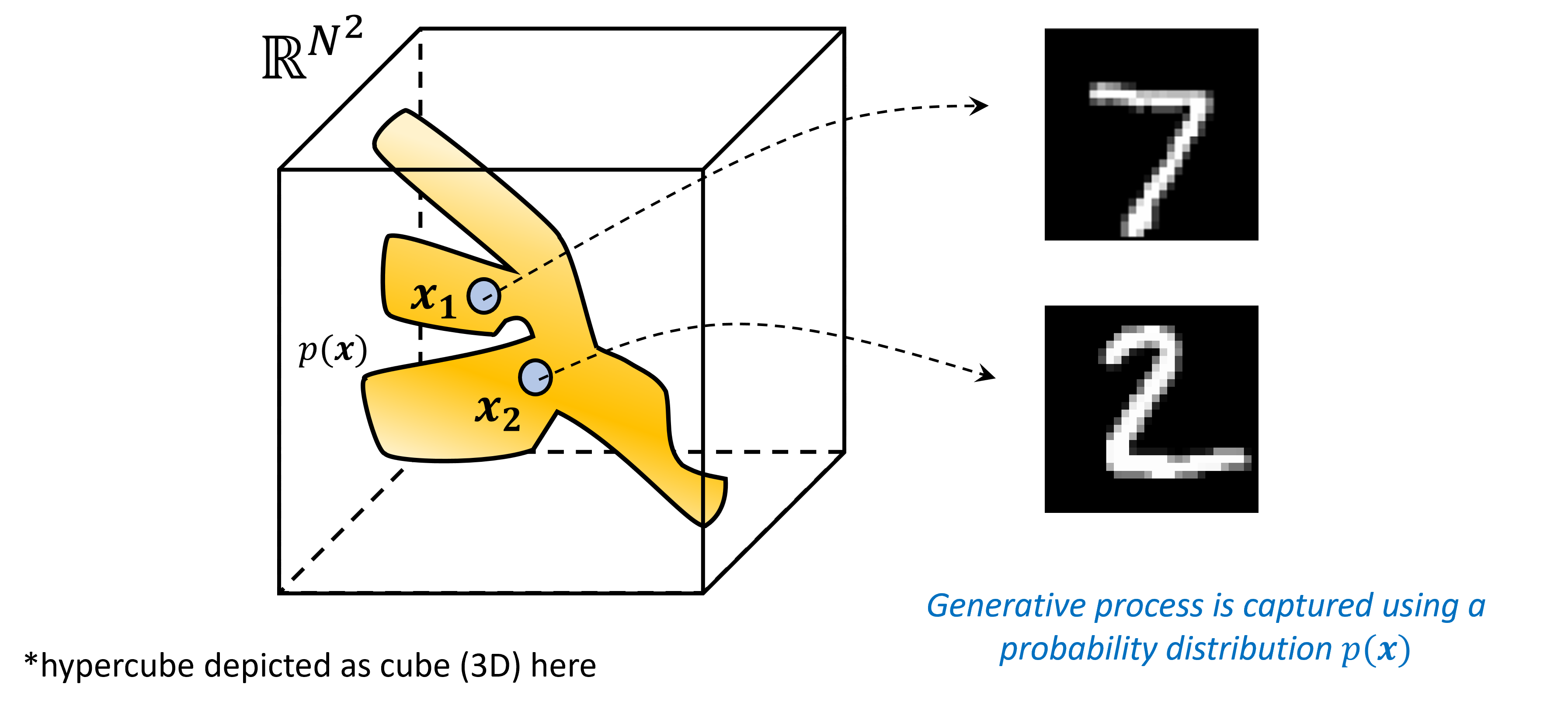
All samples on this manifold ideally coincide with samples that follow the distribution of your dataset. All the samples outside the manifold are images with any pixel configuration that does not fit your distribution. When we traverse over the manifold from one image to another, intuitively we see that the results are semantically interpolated. This is because the manifold is a non-linear function of the data. It can interpolate between samples that are not directly connected in the data space. This is a very powerful property, because it allows us to generate new data that is not in our dataset, but is still semantically similar to the data that we have. Compare this to linearly traversing between two images in the data space. This would result in very unnatural samples, that are simply the result of linearly interpolating between the images in Euclidean space.

The question remains how we can learn these complex manifolds from our dataset. And say we have been able to capture the distribution of our data. How can we now sample and generate new data from this distribution? This is what generative modeling is all about. Specifically, deep generative modeling has been proven to be very powerful in cases where your data is high-dimensional, such as images (i.e. many pixels). Examples of deep generative models are variational autoencoders (VAEs), generative adversarial networks (GANs), and normalizing flows (NFs). In this post, we will focus on a more recent addition to the family of deep generative models, namely diffusion models, also known as score-based generative models.

Diffusion models

There are already many good blogs explaining diffusion models. This post focuses on diffusion models in inverse problem solving and specifically removing structured noise. To do so, I will also start with some basics of diffusion modeling. For a complete picture, I would recommend reading some of the links at the end of this post.

Diffusion models are known for generating data from noise. Imagine starting with an image from your dataset, and gradually adding noise to it, until it becomes completely unrecognizable. Going back to our manifold story, start with a sample on the manifold, and gradually move away from it by going on a random walk (most likely falling off the manifold). This concept is borrowed from physics, where the random motion of molecules can be described with a diffusion process. Particles move from higher densities to lower densities, following the gradient of concentration. The idea of diffusion models is to learn the function that can reverse this diffusion process. Going from a random sample back to the data manifold. This function is called the score function, and it is the gradient of the log-likelihood of the data with respect to the data itself:

$$ \begin{equation} \text{score} \equiv \nabla_{\mathbf{x}} \log p\left(\mathbf{x}\right) \end{equation} $$

Quite sensibly, this score points back to our manifold, and thus can “guide” a random sample back to a sample from our desired distribution.

Diffusion models indirectly learn the data distribution using this score function. Indirectly, since we are not modeling $p(x)$ directly, but rather its gradient (the score). It comes with some advantages; namely that the score function, unlike a density, does not have to be normalized (see a more extensive story behind that here). Parameterizing densities with neural networks is a notoriously difficult task because the normalizing constant is usually intractable. Each family of deep generative models handles this differently: VAEs optimize a lower bound on the log-likelihood, GANs implicitly represent distributions by modeling the sampling process, and NFs restrict their architectures such that exact log-likelihood computation is possible. Diffusion models, on the other hand, do not have to worry about this, because they do not need to parameterize a density. In practice, this means we can use any neural network architecture for training our score. Furthermore, there are well-established techniques for learning the score function, such as denoising score matching.

Denoising score matching

Score matching techniques aim to find the optimal parameters $\theta$ of a parameterized function $s_\theta(\mathbf{x})$ such that it matches the true score $\nabla_{\mathbf{x}} \log p\left(\mathbf{x}\right)$ of our distribution as close as possible. This can be achieved using a technique named denoising score matching, where the “true score” is approximated through a denoising problem. The objective is as follows:

$$ \begin{aligned} \theta^* & =\arg \min _\theta \mathbb{E}_{\mathbf{x} \sim p_{\text {data }}(\mathbf{x})} \mathbb{E}_{\tilde{\mathbf{x}} \sim p_\sigma(\tilde{\mathbf{x}} \mid \mathbf{x})}\left[\left|s_\theta(\tilde{\mathbf{x}}, \sigma)-\nabla_{\tilde{\mathbf{x}}} \log p_\sigma(\tilde{\mathbf{x}} \mid \mathbf{x})\right|_2^2\right] \\ & =\arg \min _\theta \mathbb{E}_{\mathbf{x} \sim p_{\text {data }}(\mathbf{x})} \mathbb{E}_{\tilde{\mathbf{x}} \sim p_\sigma(\tilde{\mathbf{x}} \mid \mathbf{x})}\left[\left|s_\theta(\tilde{\mathbf{x}}, \sigma)-\frac{\mathbf{x}-\tilde{\mathbf{x}}}{\sigma^2}\right|_2^2\right] \\ & =\arg \min _\theta \mathbb{E}_{\mathbf{x} \sim p_{\text {data }}(\mathbf{x})} \mathbb{E}_{\tilde{\mathbf{x}} \sim p_\sigma(\tilde{\mathbf{x}} \mid \mathbf{x})} \operatorname{MSE}\left(s_\theta(\tilde{\mathbf{x}}, \sigma), \frac{\mathbf{x}-\tilde{\mathbf{x}}}{\sigma^2}\right) \end{aligned} $$

Let’s break this up. First, we sample a clean sample $\mathbf{x}$ from our dataset $p_{\text{data}}$. Then, we nudge this sample away from the manifold using a Gaussian kernel with mean $\mathbf{x}$ and standard deviation $\sigma$, resulting in a noisy sample $\tilde{\mathbf{x}}$ from the distribution $p_\sigma(\tilde{\mathbf{x}} \mid \mathbf{x})$. The score of this noisy sample is then given by the gradient of the log-likelihood of the noisy sample given the clean sample. Since this distribution is Gaussian, the derivative can be analytically derived, resulting in this simple MSE loss function. Furthermore, the two expectations denote that we would like to minimize this loss for all possible samples $\mathbf{x}$ in our dataset $p_{\text{data}}$, and for all possible perturbations $\tilde{\mathbf{x}}$ of our clean sample $\mathbf{x}$, given the perturbation kernel $p_\sigma$.

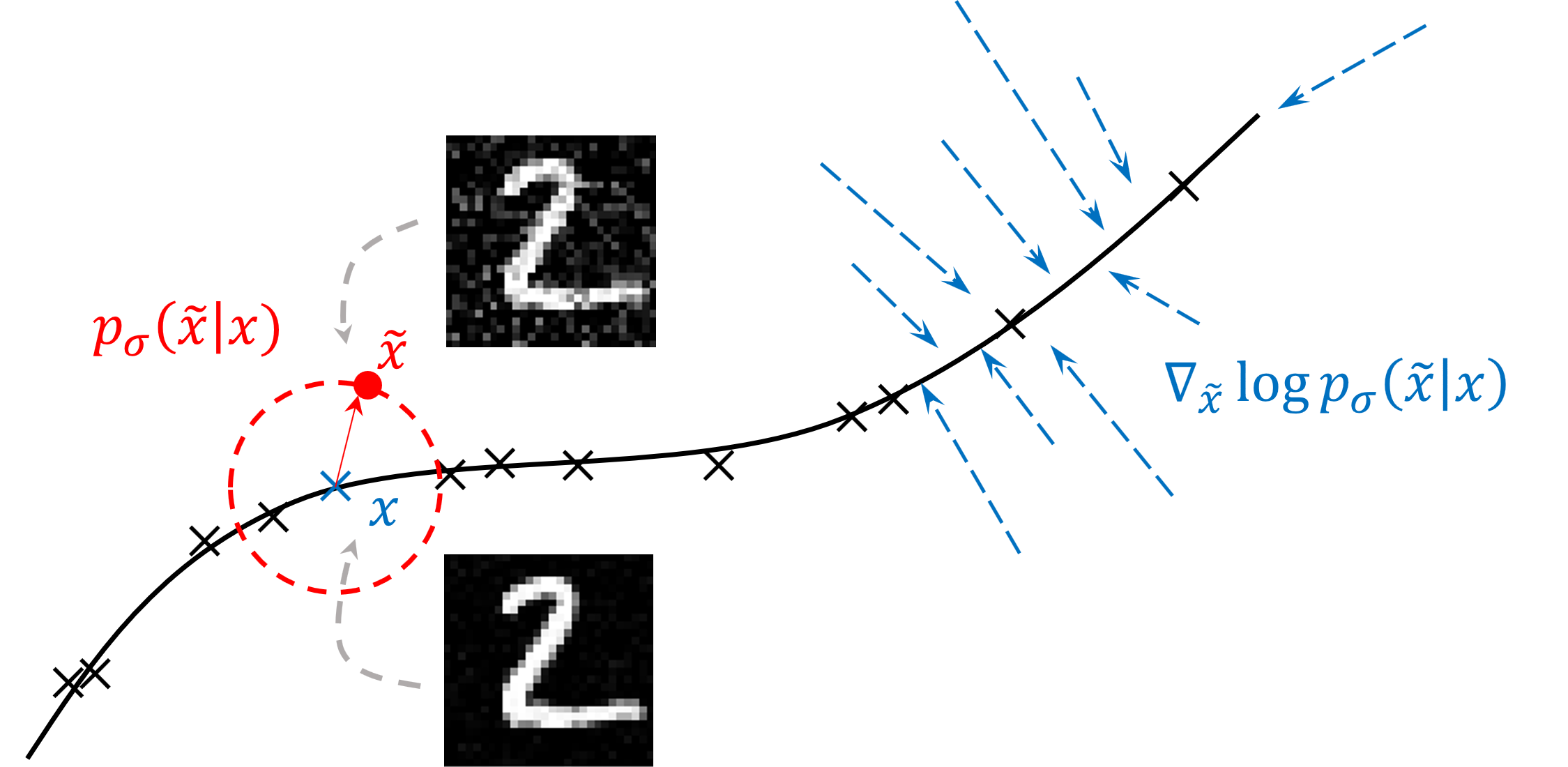
This figure shows a segment of the data manifold in 2D. The red dot represents the noisy sample $\tilde{\mathbf{x}}$, and the blue cross represents its corresponding clean sample. The gradient of the log-likelihood (score) is represented by the arrows, pointing in the direction of maximum likelihood increase. The loss function is the squared distance between our estimated score function and the gradient of the log-likelihood. Intuitively, this results in a function $s_\theta(\mathbf{x})$ that given a noisy sample, outputs a vector that points back towards its clean counterpart and thus can act as a denoising mechanism. From a density perspective, this score function can guide a random sample back to a sample from our desired distribution.

Diffusion processes

Now we have been able to train a proper score function, the next step is to define a diffusion process (remember, diffusion models aim to generate data from noise, and thus we need a mathematical way of defining that corruption process). There are several approaches to modeling a diffusion process. The approach that I personally find quite elegant and also embraces the score perspective, makes use of stochastic differential equations (SDE). An SDE is a mathematical model used to describe random processes that evolve over time. In our case, the SDE basically is an update rule for our sample $\mathbf{x}$ from one-time step in the diffusion process to another, and given by:

$$ \begin{equation} \mathrm{d} \mathbf{x}_t=f(t) \mathbf{x}_t \mathrm{~d} t+g(t) d \mathbf{w}_t, \quad t \in[0,1] \end{equation} $$

where $\mathbf{x}_1$ is a random sample from a Gaussian distribution and $\mathbf{x}_0$ a sample from our data distribution. $f(t)$ and $g(t)$ are the drift and diffusion coefficients respectively. They govern how exactly we diffuse our samples over time. The drift coefficient contributes to the deterministic part of the diffusion process, whereas the diffusion coefficient is the stochastic factor, weighing the Brownian motion process $\mathbf{w}$. Together, these two (affine) functions of time govern the noise scales of our diffusion process. To this date, these coefficients are often chosen arbitrarily, or maybe empirically if you will.

The diffusion process can now be used to gradually (this is a continuous equation) corrupt our samples into oblivion.

One property of SDEs is that, given some assumptions, they can be reversed, resulting in a reverse stochastic differential equation:

$$ \begin{equation} \mathrm{d} \mathbf{x}_t=[f(t) \mathbf{x}_t-g(t)^2 \underbrace{\nabla_{\mathbf{x}_t} \log p \left(\mathbf{x}_t\right)}_{\mathrm{score}}] \mathrm{d} t+g(t) \mathrm{d} \overline{\mathbf{w}}, \quad t \in[1,0] \end{equation} $$

Emerging from this reverse SDE is the score function. All other parameters in this diffusion process are known. Given that we have a nicely trained score function, we now have a way of getting a data sample from noise.

Let’s summarize what we have so far:

• We have the learned score function $s_\theta(\mathbf{x}) \approx \nabla_{\mathbf{x}} \log p(\mathbf{x})$
• We have a formulation (reverse SDE) for the data generation process
• We still need a numerical solver to draw samples from $p(\mathbf{x})$

Sampling with diffusion models

The diffusion process we have defined using SDEs is a continuous process. To sample from our distribution, we need to discretize this reverse diffusion process. This is done by solving the SDE for a fixed number of steps $N$, resulting in a discrete process. Luckily for us, there are already several SDE solvers out there. One of the simpler ones is the Euler-Maruyama method. The update rule for the Euler-Maruyama method is given by:

$$ \begin{equation} \mathbf{x}_{t - \Delta t} \leftarrow \mathbf{x}_t + [f(t)\mathbf{x}_t - g^2(t) s_\theta(\mathbf{x}_t)]\Delta t + g(t) \sqrt{\vert\Delta t\vert}\mathbf{z}, \quad \mathbf{z} \sim \mathcal{N}\left(0, \mathbf{I}\right) \end{equation} $$

Note that this is nothing more than a discretized version of our reverse diffusion process defined earlier. Our sample $\mathbf{x}$ is iteratively updated using the score function, and a random noise term $\mathbf{z}$, which stems from the Brownian motion part of our SDE. The noise term is sampled from a standard normal distribution, and scaled by the diffusion coefficient $g(t)$. This process resembles Langeving dynamics and can be seen as a noisy form of stochastic gradient descent (SGD). We can substitute our VPSDE drift and diffusion coefficients in the update rule, resulting in:

$$ \begin{equation} \mathbf{x}_{t - \Delta t} \leftarrow \mathbf{x}_t + [\frac{1}{2} \mathbf{x}_t - s_\theta(\mathbf{x}_t)]\beta(t)\Delta t + \sqrt{\beta(t)\vert\Delta t\vert}\mathbf{z} \end{equation} $$

In any case, you are now ready to start generating samples from your learned data distribution! But wait, there is more…

Conditional sampling

Sampling from a distribution is good and all, since it can be used to generate arbitrary samples from your learned data distribution. However, we are often interested in sampling from a conditional distribution. For example, we might want to generate images of a specific class, or a specific digit. Alternatively, we might want to denoise, inpaint or interpolate images (i.e. we already have a corrupted image at hand). In all these cases, we need to sample from a conditional distribution. This is done by conditioning the diffusion process on some additional information, the observation $\mathbf{y}$. For example, we can condition on the class label, or a corrupted image. The reverse diffusion process can be modified by replacing the prior score with a posterior score to incorporate this additional information:

$$ \mathrm{d} \mathbf{x}_t=\left[f(t) \mathbf{x}_t-g(t)^2 \nabla_{\mathbf{x}_t} \log p\left(\mathbf{x}_t \mid \mathbf{y}\right)\right] \mathrm{d} t+g(t) \mathrm{d} \overline{\mathbf{w}}, \quad t \in[1,0] $$

The posterior score $\nabla_{\mathbf{x}_t}\log p\left(\mathbf{x}_t \mid \mathbf{y}\right)$ itself can be factorized into known quantitites using the Bayes’ rule for score functions:

$$ \nabla_{\mathbf{x}_t} \log p(\mathbf{x}_t \mid \mathbf{y})=\nabla_{\mathbf{x}_t} \log p(\mathbf{x}_t)+\nabla_{\mathbf{x}_t} \log p(\mathbf{y} \mid \mathbf{x}_t) $$

The first term is approximated using our trained score model, while the second term can be analytically derived from our forward model, i.e. the likelihood of $\mathbf{y}$ given $\mathbf{x}_t$ (more on that later…).

Now let’s revisit the discretization of the sampling process, but with the addition of the conditional information.

$$ \mathbf{x}_{t - \Delta t} \leftarrow \mathbf{x}_t + [f(t)\mathbf{x}_t - g^2(t) \left\{s_\theta(\mathbf{x}_t) + p(\mathbf{y}\vert \mathbf{x}_t)\right\}]\Delta t + g(t) \sqrt{\vert\Delta t\vert}\mathbf{z}, \quad \mathbf{z} \sim \mathcal{N}\left(0, \mathbf{I}\right) $$

One way to iteratively solve this conditional reverse diffusion process is by taking out the likelihood part and move this two a second update rule. We now have a score step (prior), and a likelihood step, often known as the data consistency term, as it tries to make our solution $\mathbf{x}$ consistent with our observation $\mathbf{y}$.

$$ \begin{align} \mathbf{x}_{t - \Delta t} &\leftarrow \mathbf{x}_t & +& [f(t)\mathbf{x}_t - g^2(t) s_\theta(\mathbf{x}_t)]\Delta t + g(t) \sqrt{\vert\Delta t\vert}\mathbf{z}\\ \mathbf{x}_{t - \Delta t} &\leftarrow \mathbf{x}_{t - \Delta t} &+& \lambda\nabla_{\mathbf{x}_t}\log p(\mathbf{y}\vert \mathbf{x}_t) \end{align} $$

where $\lambda$ is a hyperparameter added to weigh the likelihood properly (encompasses the variance of the noise). But wait, unlike the likelihood model $p(\mathbf{y} \vert \mathbf{x}_0)$, the noise-perturbed likelihood $p(\mathbf{y} \vert \mathbf{x}_t)$ is generally intractable. We clearly have a definition how to go from $\mathbf{x}_0\rightarrow\mathbf{y}$ (for instance (12)), but what about $\mathbf{x}_t\rightarrow\mathbf{y}$?

It turns out there is more than one way to approximate this quantity; a method proposed by Song et al. uses a Gaussian approximation of the likelihood. This variational inference procedure is used to arrive at a tractable approximation of the noise-perturbed likelihood score, given by $p(\mathbf{y}\vert \mathbf{x}_t) \approx p(\mathbf{y}\vert\mathbf{x}_{0 \vert t})$ where $\mathbf{x}_{0 \vert t}$ is the one step denoised estimate of $\mathbf{x}_0$ at timestep $t$, given by:

$$ \begin{align} \mathbf{x}_{0 \vert t} = \mathbb{E}[\mathbf{x}_0\vert\mathbf{x}_t] = \mathbf{x}_t + \sigma_t^2\nabla_{\mathbf{x}_t}\log p(\mathbf{x}_t) \approx \mathbf{x}_t + \sigma_t^2 s_\theta(\mathbf{x}_t) \end{align} $$

which is also known as the posterior mean of the reverse diffusion process. Now we have an approximation for the posterior mean, we can use it to derive the approximated noise-perturbed likelihood score (which was our initial goal). Say we are given a denoising problem of the form:

$$ \begin{equation} \mathbf{y} = \mathbf{x} + \mathbf{n}, \quad \mathbf{n}\sim \mathcal{N}(0, \sigma_n^2\mathbf{I}), \end{equation} $$

the noise-perturbed likelihood is then approximated by $\log p(\mathbf{y} \vert \mathbf{x}_t) \approx \mathcal{N}(\mathbf{x}_{0 \vert t}, \Sigma_t)$, and since this is a Gaussian distribution, we can work out its derivative with respect to $\mathbf{x}_t$ to get the likelihood score:

$$ \begin{align} \nabla_{\mathbf{x}_t}\log p(\mathbf{y}\vert \mathbf{x}_t) & \approx (\nabla_{\mathbf{x}_t}\mathbf{x}_{0 \vert t}) \Sigma_t^{-1}(\mathbf{y} - \mathbf{x}_{0\vert t})\ \end{align} $$

where $\Sigma_t$ is a chosen variance term which depends on the variance of the data distribution at timestep $t$, or in other words dependend on $\sigma_t$ and $\sigma_n$. Subsequently, we can substitute the likelihood score into the second update rule (11). Alternate this with the score function update rule (10) and we are done!

Removing structured noise

In many real-world problems, the noise source $\mathbf{n}$ is not nicely defined, such as Gaussian. In practice, the noise is often structured and follows a complex distribution. This complicates matters, as it is not straightforward anymore what the prior on the noise should be. One solution is to also learn the noise distribution with score-based models. This will result in two priors, one for our data distribution $p(\mathbf{x})$, and one for the noise distribution $p(\mathbf{n})$. We can interleave the sampling process, sampling from both distributions at the same time while also conditioning on the observation $\mathbf{y}$. This results in a joint conditional diffusion process. Besides the score updates for $\mathbf{x}$ and $\mathbf{n}$, our likelihood model $p(\mathbf{y}\vert\mathbf{x}_t, \mathbf{n}_t)\approx p(\mathbf{y}\vert\mathbf{x}_{0\vert t}, \mathbf{n}_{0\vert t})$ is now conditioned on two variables and thus we also need to add a data consistency term for the noise:

$$ \begin{align} \mathbf{n}_{t - \Delta t} &\leftarrow \mathbf{n}_{t - \Delta t} + \kappa\nabla_{\mathbf{n}_t}\log p(\mathbf{y}\vert\mathbf{x}_t, \mathbf{n}_t)\\ &\approx \mathbf{n}_{t - \Delta t} + \kappa(\nabla_{\mathbf{n}_t}\mathbf{n}_{0 \vert t}) \Sigma_t^{-1}(\mathbf{y} - \mathbf{x}_{0\vert t} - \mathbf{n}_{0\vert t}) \end{align} $$

The data consistency step for $\mathbf{x}$ will also slightly change as we now need to condition on the noise:

$$ \begin{align} \mathbf{x}_{t - \Delta t} &\leftarrow \mathbf{x}_{t - \Delta t} + \lambda\nabla_{\mathbf{x}_t}\log p(\mathbf{y}\vert\mathbf{x}_t, \mathbf{n}_t)\\ &\approx \mathbf{x}_{t - \Delta t} + \lambda(\nabla_{\mathbf{x}_t}\mathbf{x}_{0 \vert t}) \Sigma_t^{-1}(\mathbf{y} - \mathbf{x}_{0\vert t} - \mathbf{n}_{0\vert t}) \end{align} $$

We now have two hyperparameters, $\lambda$ and $\kappa$, which we can tune to get the best results. The sampling process is now interleaved, and we can sample from both distributions at the same time. This is a rather simple way to remove structured noise from images, and it works surprisingly well.

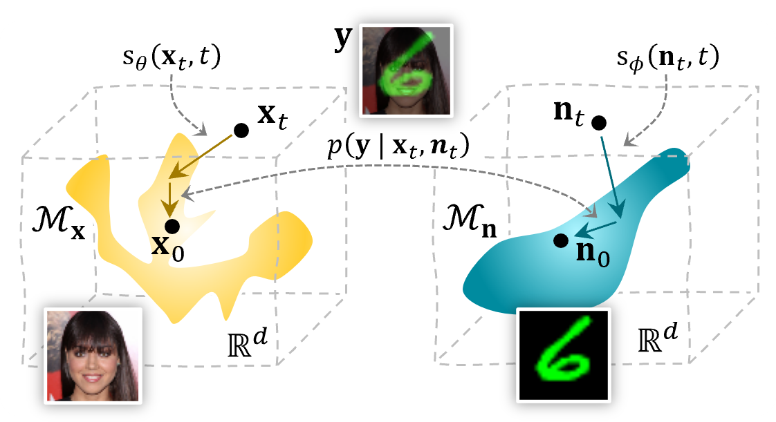Overview of the proposed joint posterior sampling method for removing structured noise using diffusion models.

Let’s test it on a rather silly setting. Some faces from the CelebA dataset will serve as our dataset, and this time we will add MNIST digits as “noise”. Obviously not Gaussian, and any method making that assumption will fail horribly trying to remove them.

Okay, show me what happens in that case (drop down)

For example, the following is a result from using our conditional inference scheme from before, with the Gaussian noise prior, but with highly structured noise:

Due to the mismatch with the actual noise and our noise prior, this method is unable to remove any of it.

Now let’s see how the structured diffusion model with a learned noise prior fares:

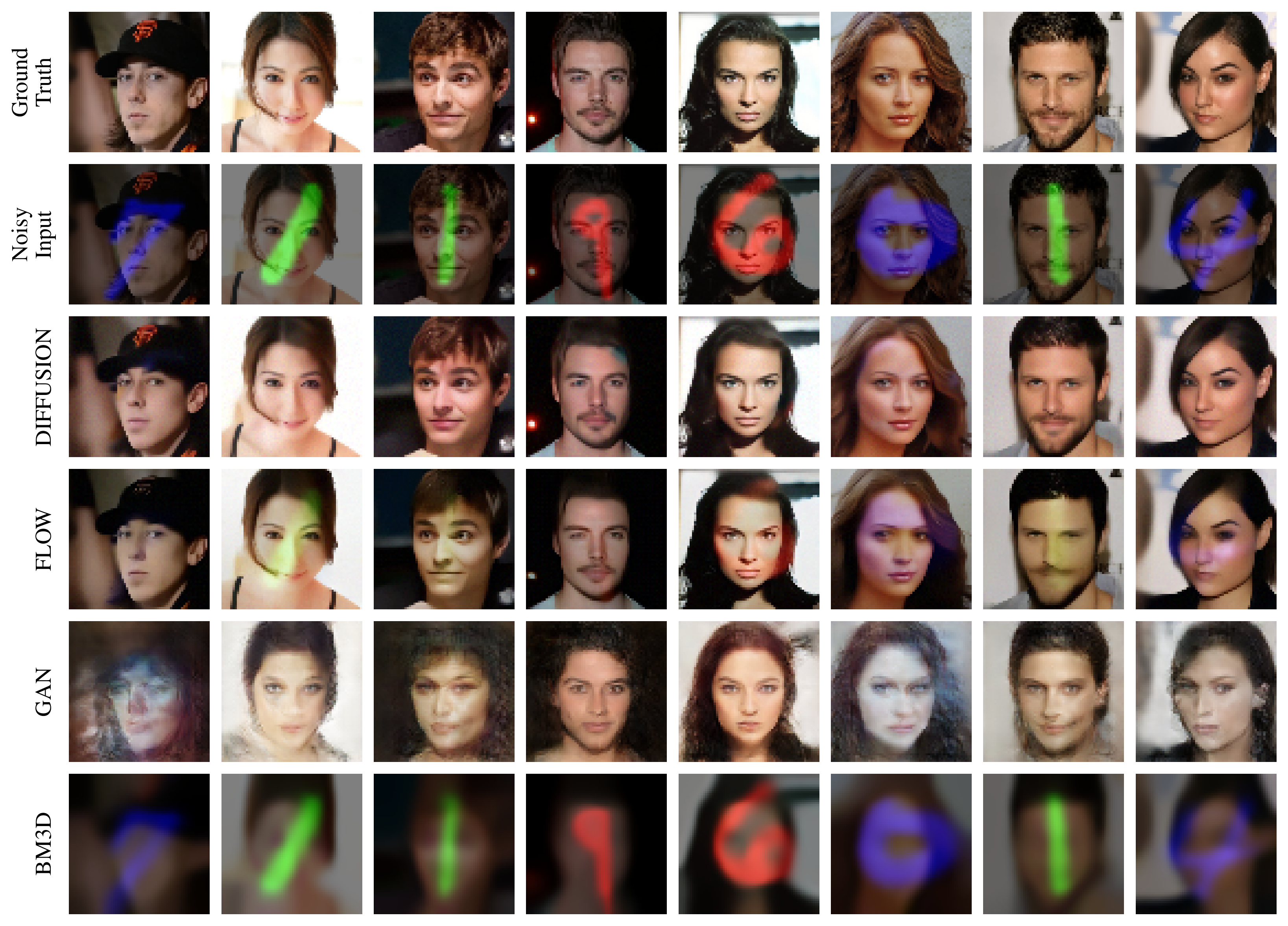
Here are some more examples, comparing the structured diffusion denoising with some other generative and non-generative methods:

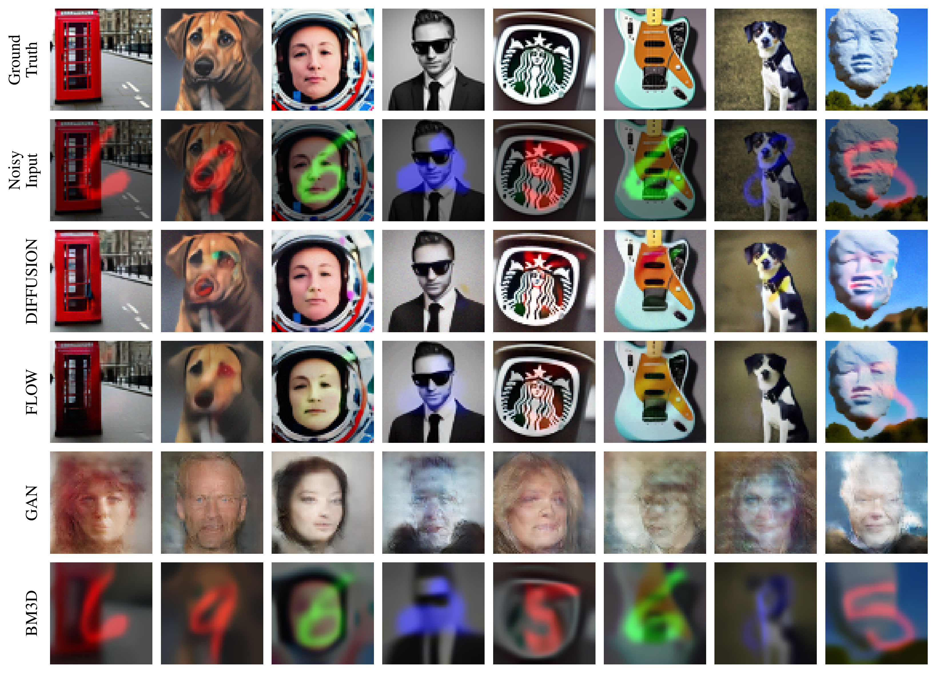
What if we test it with data that was out-of-distribution? Here I generated some random-ish images with stable diffusion and used this as the input to the denoising model.

References and reading material

• The paper that was the basis of this work: Removing Structured Noise with Diffusion Models

• Video that explains the manifold hypothesis in more detail: My understanding of the Manifold Hypothesis

• Excellent blog on original score-based diffusion model paper: Generative Modeling by Estimating Gradients of the Data Distribution

• Interesting perspective on diffusion models: Diffusion Models are Autoencoders

• Another good blog by Lilian Weng on diffusion models: What are Diffusion Models?

• Blog by Jakub Tomczak on diffusion models: Diffusion-based models

• Cool practical and simple implementation: Bare Bones Diffusion Models

• Good read on different perspectives of diffusion models: Understanding Diffusion Models: A Unified Perspective

• Even more perspectives, highlighting similarities of diffusion models with other concepts in generative modeling: Perspectives on diffusion